Training LeNet on MNIST
This tutorial goes through the code in examples/mnist to explain
the basic usage of Mocha. We will use the architecture known as
[LeNet], which is a deep convolutional neural network known to work
well on handwritten digit classification tasks. More specifically, we
will use Caffe’s modified architecture, by replacing the sigmoid
activation functions with Rectified Linear Unit (ReLU) activation
functions.
| [LeNet] | Lecun, Y.; Bottou, L.; Bengio, Y.; Haffner, P., Gradient-based learning applied to document recognition, Proceedings of the IEEE, vol.86, no.11, pp.2278-2324, Nov 1998. |
Preparing the Data
MNIST is a handwritten digit
recognition dataset containing 60,000 training examples and 10,000
test examples. Each example is a 28x28 single channel grayscale
image. The dataset can be downloaded in a binary format from Yann
LeCun’s website. We have created
a script get-mnist.sh to download the dataset, and it calls
mnist.convert.jl to convert the binary dataset into a HDF5 file that
Mocha can read.
When the conversion finishes, data/train.hdf5 and
data/test.hdf5 will be generated.
Defining the Network Architecture
The LeNet consists of a convolution layer followed by a pooling layer, and then another convolution followed by a pooling layer. After that, two densely connected layers are added. We don’t use a configuration file to define a network architecture like Caffe, instead, the network definition is directly done in Julia. First of all, let’s import the Mocha package.
using Mocha
Then we will define a data layer, which reads the HDF5 file and provides input for the network:
data_layer  = HDF5DataLayer(name="train-data", source="data/train.txt",
    batch_size=64, shuffle=true)
Note the source is a simple text file that contains a list of real
data files (in this case data/train.hdf5). This behavior is the
same as in Caffe, and could be useful when your dataset contains a lot
of files. The network processes data in mini-batches, and we are using a batch
size of 64 in this example. Larger mini-batches take more computational time but give a lower variance estimate of the loss function/gradient at each iteration. We also enable random shuffling of the data set to prevent structure in the ordering of input samples from influencing training.
Next we define a convolution layer in a similar way:
conv_layer = ConvolutionLayer(name="conv1", n_filter=20, kernel=(5,5),
    bottoms=[:data], tops=[:conv1])
There are several parameters specified here:
name- Every layer can be given a name. When saving the model to disk and loading back, this is used as an identifier to map to the correct layer. So if your layer contains learned parameters (a convolution layer contains learned filters), you should give it a unique name. It is a good practice to give every layer a unique name to get more informative debugging information when there are any potential issues.
n_filter- Number of convolution filters.
kernel- The size of each filter. This is specified in a tuple containing kernel width and kernel height, respectively. In this case, we are defining a 5x5 square filter.
bottoms- An array of symbols specifying where to get data from. In this case,
we are asking for a single data source called
:data. This is provided by the HDF5 data layer we just defined. By default, the HDF5 data layer tries to find two datasets nameddataandlabelfrom the HDF5 file, and provide two streams of data called:dataand:label, respectively. You can change that by specifying thetopsproperty for the HDF5 data layer if needed. tops- This specifies a list of names for the output of the convolution
layer. In this case, we are only taking one stream of input, and
after convolution we output one stream of convolved data with the
name
:conv1.
Another convolution layer and pooling layer are defined similarly, this time with more filters:
pool_layer = PoolingLayer(name="pool1", kernel=(2,2), stride=(2,2),
    bottoms=[:conv1], tops=[:pool1])
conv2_layer = ConvolutionLayer(name="conv2", n_filter=50, kernel=(5,5),
    bottoms=[:pool1], tops=[:conv2])
pool2_layer = PoolingLayer(name="pool2", kernel=(2,2), stride=(2,2),
    bottoms=[:conv2], tops=[:pool2])
Note how tops and bottoms define the computation or data
dependency. After the convolution and pooling layers, we add two fully
connected layers. They are called InnerProductLayer because the
computation is basically an inner product between the input and the
layer weights. The layer weights are also learned, so we also give
names to the two layers:
fc1_layer  = InnerProductLayer(name="ip1", output_dim=500,
    neuron=Neurons.ReLU(), bottoms=[:pool2], tops=[:ip1])
fc2_layer  = InnerProductLayer(name="ip2", output_dim=10,
    bottoms=[:ip1], tops=[:ip2])
Everything should be self-evident. The output_dim property of an
inner product layer specifies the dimension of the output. Note the
dimension of the input is automatically determined from the bottom
data stream.
For the first inner product layer we specify a Rectified
Linear Unit (ReLU) activation function via the neuron
property. An activation function could be added to almost any
computation layer. By default, no activation
function, or the identity activation function is used. We don’t use
activation an function for the last inner product layer, because that
layer acts as a linear classifier. For more details, see Neurons (Activation Functions).
The output dimension of the last inner product layer is 10, which corresponds to the number of classes (digits 0~9) of our problem.
This is the basic structure of LeNet. In order to train this network, we need to define a loss function. This is done by adding a loss layer:
loss_layer = SoftmaxLossLayer(name="loss", bottoms=[:ip2,:label])
Note this softmax loss layer takes as input :ip2, which is the
output of the last inner product layer, and :label, which comes
directly from the HDF5 data layer. It will compute an averaged loss
over each mini-batch, which allows us to initiate back propagation to
update network parameters.
Configuring the Backend and Building the Network
Now we have defined all the relevant layers. Let’s setup the computation backend and construct a network with those layers. In this example, we will go with the simple pure Julia CPU backend first:
backend = CPUBackend()
init(backend)
The init function of a Mocha Backend will initialize the
computation backend. With an initialized backend, we can go ahead and
construct our network:
common_layers = [conv_layer, pool_layer, conv2_layer, pool2_layer,
    fc1_layer, fc2_layer]
net = Net("MNIST-train", backend, [data_layer, common_layers..., loss_layer])
A network is built by passing the constructor an initialized backend,
and a list of layers. Note how we use common_layers to collect a
subset of the layers. This will be useful later when constructing a network to process validation data.
Configuring the Solver
We will use Stochastic Gradient Descent (SGD) to solve/train our deep network.
exp_dir = "snapshots"
method = SGD()
params = make_solver_parameters(method, max_iter=10000, regu_coef=0.0005,
    mom_policy=MomPolicy.Fixed(0.9),
    lr_policy=LRPolicy.Inv(0.01, 0.0001, 0.75),
    load_from=exp_dir)
solver = Solver(method, params)
The behavior of the solver is specified by the following parameters:
max_iter- Max number of iterations the solver will run to train the network.
regu_coef- Regularization coefficient. By default, both the convolution layer and the inner product layer have L2 regularizers for their weights (and no regularization for bias). Those regularizations could be customized for each layer individually. The parameter here is a global scaling factor for all the local regularization coefficients.
mom_policy- This specifies the momentum policy used during training. Here we are using a fixed momentum policy of 0.9 throughout training. See the Caffe document for rules of thumb for setting the learning rate and momentum.
lr_policy- The learning rate policy. In this example, we are using the
Invpolicy with gamma = 0.001 and power = 0.75. This policy will gradually shrink the learning rate, by setting it to base_lr * (1 + gamma * iter)-power. load_fromThis can be a saved model file or a directory. For the latter case, the latest saved model snapshot will be loaded automatically before the solver loop starts. We will see in a minute how to configure the solver to save snapshots automatically during training.
This is useful to recover from a crash, to continue training with a larger
max_iteror to perform fine tuning on some pre-trained models.
Coffee Breaks for the Solver
Now our solver is ready to go. But in order to give it a healthy working plan, we provide it with some coffee breaks:
setup_coffee_lounge(solver, save_into="$exp_dir/statistics.jld", every_n_iter=1000)
This sets up the coffee lounge, which holds data reported during coffee breaks. Here we also specify a file to save the information we accumulated in coffee breaks to disk. Depending on the coffee breaks, useful statistics such as objective function values during training will be saved, and can be loaded later for plotting or inspecting.
add_coffee_break(solver, TrainingSummary(), every_n_iter=100)
First, we allow the solver to have a coffee break after every
100 iterations so that it can give us a brief summary of the
training process. By default TrainingSummary will print the loss
function value on the last training mini-batch.
We also add a coffee break to save a snapshot of the trained network every 5,000 iterations:
add_coffee_break(solver, Snapshot(exp_dir), every_n_iter=5000)
Note that we are passing exp_dir to the constructor of the Snapshot coffee
break so snapshots will be saved into that directory. And according to our
configuration of the solver above, the latest snapshots will
be automatically loaded by the solver if you run this script again.
In order to see whether we are really making progress or simply overfitting, we also wish to periodically see the performance on a separate validation set. In this example, we simply use the test dataset as the validation set.
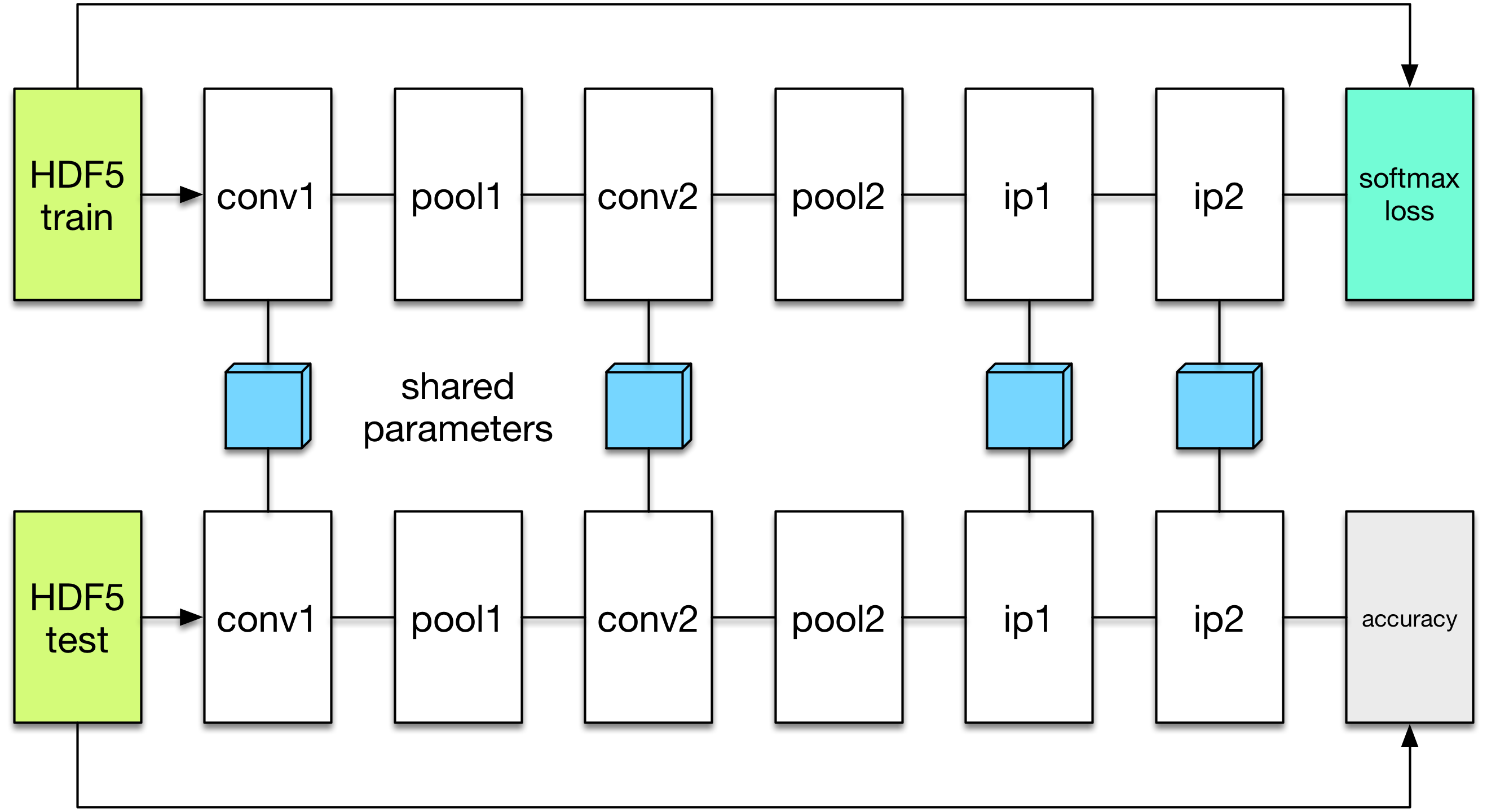
We will define a new network to perform the evaluation. The evaluation network will have exactly the same architecture, except with a different data layer that reads from the validation dataset instead of the training set. We also do not need the softmax loss layer as we will not train the validation network. Instead, we will add an accuracy layer on top, which will compute the classification accuracy.
data_layer_test = HDF5DataLayer(name="test-data", source="data/test.txt", batch_size=100)
acc_layer = AccuracyLayer(name="test-accuracy", bottoms=[:ip2, :label])
test_net = Net("MNIST-test", backend, [data_layer_test, common_layers..., acc_layer])
Note how we re-use the common_layers variable defined a earlier to re-use
the description of the network architecture. By passing the same layer objects
used to define the training net to the constructor of the validation net, Mocha
will automatically setup parameter sharing between the two networks.
The two networks will look like this:
Now we are ready to add another coffee break to report the validation performance:
add_coffee_break(solver, ValidationPerformance(test_net), every_n_iter=1000)
Please note that we use a different batch size (100) in the validation network. During the coffee break, Mocha will run exactly one epoch on the validation net (100 iterations in our case, as we have 10,000 samples in the MNIST test set), and report the average classification accuracy. You do not need to specify the number of iterations here as the HDF5 data layer will report the epoch number as it goes through a full pass of the dataset.
Training
Without further ado, we can finally start the training process:
solve(solver, net)

destroy(net)
destroy(test_net)
shutdown(backend)
After training, we will shutdown the system to release all the allocated resources. Now you are ready run the script:
julia mnist.jl
As training proceeds, progress information will be reported. It takes about 10~20 seconds every 100 iterations, i.e. about 7 iterations per second, on my machine, depending on the server load and many other factors.
14-Nov 11:56:13:INFO:root:001700 :: TRAIN obj-val = 0.43609169
14-Nov 11:56:36:INFO:root:001800 :: TRAIN obj-val = 0.21899594
14-Nov 11:56:58:INFO:root:001900 :: TRAIN obj-val = 0.19962406
14-Nov 11:57:21:INFO:root:002000 :: TRAIN obj-val = 0.06982464
14-Nov 11:57:40:INFO:root:
14-Nov 11:57:40:INFO:root:## Performance on Validation Set
14-Nov 11:57:40:INFO:root:---------------------------------------------------------
14-Nov 11:57:40:INFO:root:  Accuracy (avg over 10000) = 96.0500%
14-Nov 11:57:40:INFO:root:---------------------------------------------------------
14-Nov 11:57:40:INFO:root:
14-Nov 11:58:01:INFO:root:002100 :: TRAIN obj-val = 0.18091436
14-Nov 11:58:21:INFO:root:002200 :: TRAIN obj-val = 0.14225903
The training could run faster by enabling the native extension for the CPU backend, or by using the CUDA backend if CUDA compatible GPU devices are available. Please refer to Mocha Backends for how to use different backends.
Just to give you a feeling for the potential speed improvement, this is a sample log from running with the Native Extension enabled CPU backend. It runs at about 20 iterations per second.
14-Nov 12:15:56:INFO:root:001700 :: TRAIN obj-val = 0.82937032
14-Nov 12:16:01:INFO:root:001800 :: TRAIN obj-val = 0.35497263
14-Nov 12:16:06:INFO:root:001900 :: TRAIN obj-val = 0.31351241
14-Nov 12:16:11:INFO:root:002000 :: TRAIN obj-val = 0.10048970
14-Nov 12:16:14:INFO:root:
14-Nov 12:16:14:INFO:root:## Performance on Validation Set
14-Nov 12:16:14:INFO:root:---------------------------------------------------------
14-Nov 12:16:14:INFO:root:  Accuracy (avg over 10000) = 94.5700%
14-Nov 12:16:14:INFO:root:---------------------------------------------------------
14-Nov 12:16:14:INFO:root:
14-Nov 12:16:18:INFO:root:002100 :: TRAIN obj-val = 0.20689486
14-Nov 12:16:23:INFO:root:002200 :: TRAIN obj-val = 0.17757215
The following is a sample log from running with the CUDA backend. It runs at about 300 iterations per second.
14-Nov 12:57:07:INFO:root:001700 :: TRAIN obj-val = 0.33347249
14-Nov 12:57:07:INFO:root:001800 :: TRAIN obj-val = 0.16477060
14-Nov 12:57:07:INFO:root:001900 :: TRAIN obj-val = 0.18155883
14-Nov 12:57:08:INFO:root:002000 :: TRAIN obj-val = 0.06635486
14-Nov 12:57:08:INFO:root:
14-Nov 12:57:08:INFO:root:## Performance on Validation Set
14-Nov 12:57:08:INFO:root:---------------------------------------------------------
14-Nov 12:57:08:INFO:root:  Accuracy (avg over 10000) = 96.2200%
14-Nov 12:57:08:INFO:root:---------------------------------------------------------
14-Nov 12:57:08:INFO:root:
14-Nov 12:57:08:INFO:root:002100 :: TRAIN obj-val = 0.20724633
14-Nov 12:57:08:INFO:root:002200 :: TRAIN obj-val = 0.14952177
The accuracy from two different training runs are different due to different random initializations. The objective function values shown here are also slightly different from Caffe’s, as until recently, Mocha counts regularizers in the forward stage and adds them into the objective functions. This behavior is removed in more recent versions of Mocha to avoid unnecessary computations.
Using Saved Snapshots for Prediction
Often you want to use a network previously trained with Mocha to make individual predictions. Earlier during the training process snapshots of the network state were saved every 5000 iterations, and these can be reloaded at a later time. To do this we first need a network with the same shape and configuration as the one used for training, except instead we supply a MemoryDataLayer instead of a HDF5DataLayer, and a SoftmaxLayer instead of a SoftmaxLossLayer:
using Mocha
backend = CPUBackend()
init(backend)

mem_data = MemoryDataLayer(name="data", tops=[:data], batch_size=1,
    data=Array[zeros(Float32, 28, 28, 1, 1)])
softmax_layer = SoftmaxLayer(name="prob", tops=[:prob], bottoms=[:ip2])

# define common_layers as earlier

run_net = Net("imagenet", backend, [mem_data, common_layers..., softmax_layer])
Note that common_layers has the same definition as above, and that we specifically pass a Float32 array to the MemoryDataLayer so that it will match the Float32 data type used in the MNIST HDF5 training dataset. Next we fill in this network with the learned parameters from the final training snapshot:
load_snapshot(run_net, "snapshots/snapshot-010000.jld")
Now we are ready to make predictions using our trained model. A simple way to accomplish this is to take the first test data point and run it through the model. This is done by setting the data of the MemoryDataLayer to the first test image and then using forward to execute the network. Note that the labels in the test data are indexed starting with 0 not 1 so we adjust them before printing.
using HDF5
h5open("data/test.hdf5") do f
    get_layer(run_net, "data").data[1][:,:,1,1] = f["data"][:,:,1,1]
    println("Correct label index: ", Int64(f["label"][:,1][1]+1))
end

forward(run_net)
println()
println("Label probability vector:")
println(run_net.output_blobs[:prob].data)
This produces the output:
Correct label index: 5

Label probability vector:
Float32[5.870685e-6
        0.00057068263
        1.5419962e-5
        8.387835e-7
        0.99935246
        5.5915066e-6
        4.284061e-5
        1.2896479e-6
        4.2869314e-7
        4.600691e-6]
Checking The Solver’s Progress with Learning Curves
While a network is training we should verify that the optimization of the weights and biases is converging to a solution. One of the best ways to do this is to plot the Learning Curve as the solver progresses through its iterations. A neural network’s Learning Curve is a plot of iterations along the \(x\) axis and the value of the objective function along the \(y\) axis. Recall that the solver is trying to minimize the objective function so the value plotted along the \(y\) axis should decrease over time. The image below inludes the raw data from the neural network in this tutorial and a smoothed plot that uses a low pass filter of the data to take out high frequency noise. More about noise in stochastic gradient descent later. For now let’s focus on generating a Learning Curve like the one here.
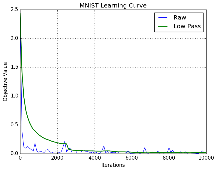
Verifying convergence after a few thousand iterations is essential when developing neural networks on new datasets. Some teams have waited hours (or days) for their network to complete training only to discover that the solver failed to converge and they need to retune their paramaters. A quick look at the learning curve above after the first thousand iterations clearly shows that the algorithm is working and that letting it continue to train for the full 10,000 iterations will probably produce a good result.
The data to plot the Learning Curve is conveniently saved as the solver progresses. Recall that we set up the coffee lounge and a TrainingSummary() coffee break every 100 iterations in the mnist.jl file:
exp_dir = "snapshots"
setup_coffee_lounge(solver, save_into="$exp_dir/statistics.jld", every_n_iter=1000)
add_coffee_break(solver, TrainingSummary(), every_n_iter=100)
Given this data we can write a new Julia script to read the statistics.jld file and plot the learning curve while the solver continues to work. The source code for plotting the learning curve is included in the examples folder and called mnist_learning_curve.jl.
In order to see the plot we need to use a plotting package. The PyPlot package that implements matplotlib for Julia is adequate for this. Use the standard Pkg.add("PyPlot") if you do not already have it. We will also need to load the statistics.jld file using Julia’s implementation of the HDF5 format which requires the JLD packge.
using PyPlot, JLD
Next, we need to load the data. This is not difficult, but requires some careful handling because the statistics.jld file is a Julia Dict that includes several sub-dictionaries. You may need to adjust the path in the load("snapshots/statistics.jld") command so that it accurately reflects the path from where the code is running to the snapshots directory.
stats = load("snapshots/statistics.jld")
# println(typeof(stats))

tables = stats["statistics"]
ov = tables["obj_val"]
xy = sort(collect(ov))
x = [i for (i,j) in xy]
y = [j for (i,j) in xy]
x = convert(Array{Int64}, x)
y = convert(Array{Float64}, y)
From the code above we can see that the obj_val dictionary is available in the snapshot. This dictionary gets appended every 100 iterations when the solver records a TrainingSummary(). Then those values get written to disk every 1000 iterations when the solve heads out to the coffee lounge for a break. Also note that stats is not a filehandle opened to the statistics file. It is a Dict{ByteString,Any}. This is desired because we do not want the learning curve script to lock out the mnist.jl script from getting file handle access to the snapshots files. You can uncomment println(typeof(stats)) to verify that we do not have a file handle. At the end of this snippet we have a vector for \(x\) and \(y\). Now we need to plot them which is simply handled in the snippet below.
raw = plot(x, y, linewidth=1, label="Raw")
xlabel("Iterations")
ylabel("Objective Value")
title("MNIST Learning Curve")
grid("on")
The last thing we need to talk about is the noise we see in the blue line in the plot above. Recall that we chose stochastic gradient descent (SGD) as the network solver in this line from the mnist.jl file:
method = SGD()
In pure gradient descent the solution moves closer to a minima each and every step; however, in order for the solver to do this it must compute the objective function for every training sample on each step. In our case this would mean all 50,000 training samples must be processed through the network to compute the loss for one iteration of gradient descent. This is computationally expensive and slow. Stochastic gradient descent avoids this performance penalty by computing the loss function on a subset of the training examples (batches of 64 in this example). The downside of using SGD is that it sometimes takes steps in the wrong direction since it is optimizing globally on a small subset of the training examples. These missteps create the noise in the blue line. Therefore, we also create a plot that has been through a low pass filter to take out the noise which reveals the trend in the objective function.
function low_pass{T <: Real}(x::Vector{T}, window::Int)
    len = length(x)
    y = Vector{Float64}(len)
    for i in 1:len
        # I want the mean of the first i terms up to width of window
        # Putting some numbers to this with window 4
        # i win lo  hi
        # 1  4  1   1
        # 2  4  1   2
        # 3  4  1   3
        # 4  4  1   4
        # 5  4  1   5
        # 6  4  2   6  => window starts to slide
        lo = max(1, i - window)
        hi = i
        y[i] = mean(x[lo:hi])
    end
    return y
end
There are other (purer) ways to implement a low pass filter but this is adequate to create a smoothed curve for analyzing the global direction of network training. One appealing heuristics of this filter is that it outputs a solution for the first few data points consistent with the raw plot. With the filter we can now generate a smoothed set of \(y\) datapoints.
window = Int64(round(length(xy)/4.0))
y_avg = low_pass(y, window)
avg = plot(x, y_avg, linewidth=2, label="Low Pass")
legend(handles=[raw; avg])
show()  #required to display the figure in non-interactive mode
We declare window to be about one-quarter the length of the input to enforce a lot of smoothing. Also note that we use the labels to create a legend on the graph. Finally, this example places the low_pass function in the middle of the script which is not best practice, but the order presented here felt most appropriate for thinking through the different elements of the example.
There are lots of great resources on the web for building and training neural networks and after this example you now know how to use Julia and Mocha to contruct, train, and validate one of the most famous convolutional neural networks.
Thank you for working all the way to the end of the MNIST tutorial!