Training LeNet on MNIST
This tutorial goes through the code in examples/mnist to explain
the basic usages of Mocha. We will use the architecture known as
[LeNet], which is a deep convolutional neural network known to work
well on handwritten digit classification tasks. More specifically, we
will use Caffe’s modified architecture, by replacing the sigmoid
activation functions with Rectified Learning Unit (ReLU) activation
functions.
| [LeNet] | Lecun, Y.; Bottou, L.; Bengio, Y.; Haffner, P., Gradient-based learning applied to document recognition, Proceedings of the IEEE, vol.86, no.11, pp.2278-2324, Nov 1998. |
Preparing the Data
MNIST is a handwritten digit
recognition dataset containing 60,000 training examples and 10,000
test examples. Each example is a 28x28 single channel grayscale
image. The dataset in a binary format could be downloaded from Yann
LeCun’s website. We have created
a script get-mnist.sh to download the dataset, and it will call
mnist.convert.jl to convert the binary dataset into a HDF5 file that
Mocha can read.
When the conversion finishes, data/train.hdf5 and
data/test.hdf5 will be generated.
Defining the Network Architecture
The LeNet consists of a convolution layer followed by a pooling layer, and then another convolution followed by a pooling layer. After that, two densely connected layers were added. We don’t use a configuration file to define a network architecture like Caffe, instead, the network definition is directly done in Julia. First of all, let’s import the Mocha package.
using Mocha
Then we will define a data layer, which reads the HDF5 file and provides input for the network:
data_layer  = HDF5DataLayer(name="train-data", source="data/train.txt",
    batch_size=64, shuffle=true)
Note the source is a simple text file that contains a list of real
data files (in this case data/train.hdf5). This behavior is the
same as in Caffe, and could be useful when your dataset contains a lot
of files. The network processes data in mini-batches, and we are using a batch
size of 64 in this example. We also enable random shuffling of the data set.
Next we define a convolution layer in a similar way:
conv_layer = ConvolutionLayer(name="conv1", n_filter=20, kernel=(5,5),
    bottoms=[:data], tops=[:conv])
There are more parameters we specified here
name- Every layer can be given a name. When saving the model to disk and loading back, this is used as an identifier to map to the correct layer. So if your layer contains learned parameters (a convolution layer contains learned filters), you should give it a unique name. It is a good practice to give every layer a unique name, for the purpose of getting more informative debugging information when there are any potential issues.
n_filter- Number of convolution filters.
kernel- The size of each filter. This is specified in a tuple containing kernel width and kernel height, respectively. In this case, we are defining a 5x5 square filter size.
bottoms- An array of symbols specifying where to get data from. In this case,
we are asking for a single data source called
:data. This is provided by the HDF5 data layer we just defined. By default, the HDF5 data layer tries to find two datasets nameddataandlabelfrom the HDF5 file, and to provide two streams of data called:dataand:label, respectively. You can change that by specifying thetopsproperty for the HDF5 data layer if needed. tops- This specifies a list of names for the output of the convolution
layer. In this case, we are only taking one stream of input and
after convolution, we output one stream of convolved data with the
name
:conv.
Another convolution layer and pooling layer are defined similarly, with more filters this time:
pool_layer = PoolingLayer(name="pool1", kernel=(2,2), stride=(2,2),
    bottoms=[:conv], tops=[:pool])
conv2_layer = ConvolutionLayer(name="conv2", n_filter=50, kernel=(5,5),
    bottoms=[:pool], tops=[:conv2])
pool2_layer = PoolingLayer(name="pool2", kernel=(2,2), stride=(2,2),
    bottoms=[:conv2], tops=[:pool2])
Note how tops and bottoms define the computation or data
dependency. After the convolution and pooling layers, we add two fully
connected layers. They are called InnerProductLayer because the
computation is basically inner products between the input and the
layer weights. The layer weights are also learned, so we also give
names to the two layers:
fc1_layer  = InnerProductLayer(name="ip1", output_dim=500,
    neuron=Neurons.ReLU(), bottoms=[:pool2], tops=[:ip1])
fc2_layer  = InnerProductLayer(name="ip2", output_dim=10,
    bottoms=[:ip1], tops=[:ip2])
Everything should be self-evident. The output_dim property of an
inner product layer specifies the dimension of the output. Note the
dimension of the input is automatically determined from the bottom
data stream.
Note for the first inner product layer, we specifies a Rectified
Learning Unit (ReLU) activation function via the neuron
property. An activation function could be added to almost all
computation layers. By default, no activation
function, or the identity activation function is used. We don’t use
activation function for the last inner product layer, because that
layer acts as a linear classifier. For more details, see Neurons (Activation Functions).
The output dimension of the last inner product layer is 10, which corresponds to the number of classes (digits 0~9) of our problem.
This is the basic structure of LeNet. In order to train this network, we need to define a loss function. This is done by adding a loss layer:
loss_layer = SoftmaxLossLayer(name="loss", bottoms=[:ip2,:label])
Note this softmax loss layer takes as input :ip2, which is the
output of the last inner product layer, and :label, which comes
directly from the HDF5 data layer. It will compute an averaged loss
over each mini batch, which allows us to initiate back propagation to
update network parameters.
Configuring the Backend and Building the Network
Now we have defined all the relevant layers. Let’s setup the computation backend and construct a network with those layers. In this example, we will go with the simple pure Julia CPU backend first:
backend = CPUBackend()
The init function of a Mocha Backend will initialize the
computation backend. With an initialized backend, we can go ahead and
construct our network:
common_layers = [conv_layer, pool_layer, conv2_layer, pool2_layer,
    fc1_layer, fc2_layer]
net = Net("MNIST-train", backend, [data_layer, common_layers..., loss_layer])
A network is built by passing the constructor an initialized backend,
and a list of layers. Note how we use common_layers to collect a
subset of the layers. We will explain this in a minute.
Configuring the Solver
We will use Stochastic Gradient Descent (SGD) to solve or train our deep network.
exp_dir = "snapshots"

params = SolverParameters(max_iter=10000, regu_coef=0.0005,
    mom_policy=MomPolicy.Fixed(0.9),
    lr_policy=LRPolicy.Inv(0.01, 0.0001, 0.75),
    load_from=exp_dir)
solver = SGD(params)
The behavior of the solver is specified in the following parameters
max_iter- Max number of iterations the solver will run to train the network.
regu_coef- Regularization coefficient. By default, both the convolution layer and the inner product layer have L2 regularizers for their weights (and no regularization for bias). Those regularizations could be customized for each layer individually. The parameter here is just a global scaling factor for all the local regularization coefficients if any.
mom_policy- This specifies the policy of setting the momentum during training. Here we are using a policy that simply uses a fixed momentum of 0.9 all the time. See the Caffe document for rules of thumb for setting the learning rate and momentum.
lr_policy- The learning rate policy. In this example, we are using the
Invpolicy with gamma = 0.001 and power = 0.75. This policy will gradually shrink the learning rate, by setting it to base_lr * (1 + gamma * iter)-power. load_fromThis could be a file of a saved model or a directory. For the latter case, the latest saved model snapshot will be loaded automatically before the solver loop starts. We will see in a minute how to configure the solver to save snapshots automatically during training.
This is useful to recover from a crash, to continue training with a larger
max_iteror to perform fine tuning on some pre-trained models.
Coffee Breaks for the Solver
Now our solver is ready to go. But in order to give it a healthy working plan, we provide it with some coffee breaks:
setup_coffee_lounge(solver, save_into="$exp_dir/statistics.hdf5", every_n_iter=1000)
This sets up the coffee lounge. It also specifies a file to save the information we accumulated in coffee breaks. Depending on the coffee breaks, useful statistics like objective function values during training will be saved into that file, and can be loaded later for plotting or inspecting.
add_coffee_break(solver, TrainingSummary(), every_n_iter=100)
First of all, we allow the solver to have a coffee break after every
100 iterations so that it can give us a brief summary of the
training process. Currently TrainingSummary will print the loss
function value on the last training mini-batch.
We also add a coffee break to save a snapshot for the trained network every 5,000 iterations.
add_coffee_break(solver, Snapshot(exp_dir), every_n_iter=5000)
Note that we are passing exp_dir to the constructor of the Snapshot coffee
break. The snapshots will be saved into that directory. And according to our
configuration of the solver above, the latest snapshots will
be automatically loaded by the solver if you run this script again.
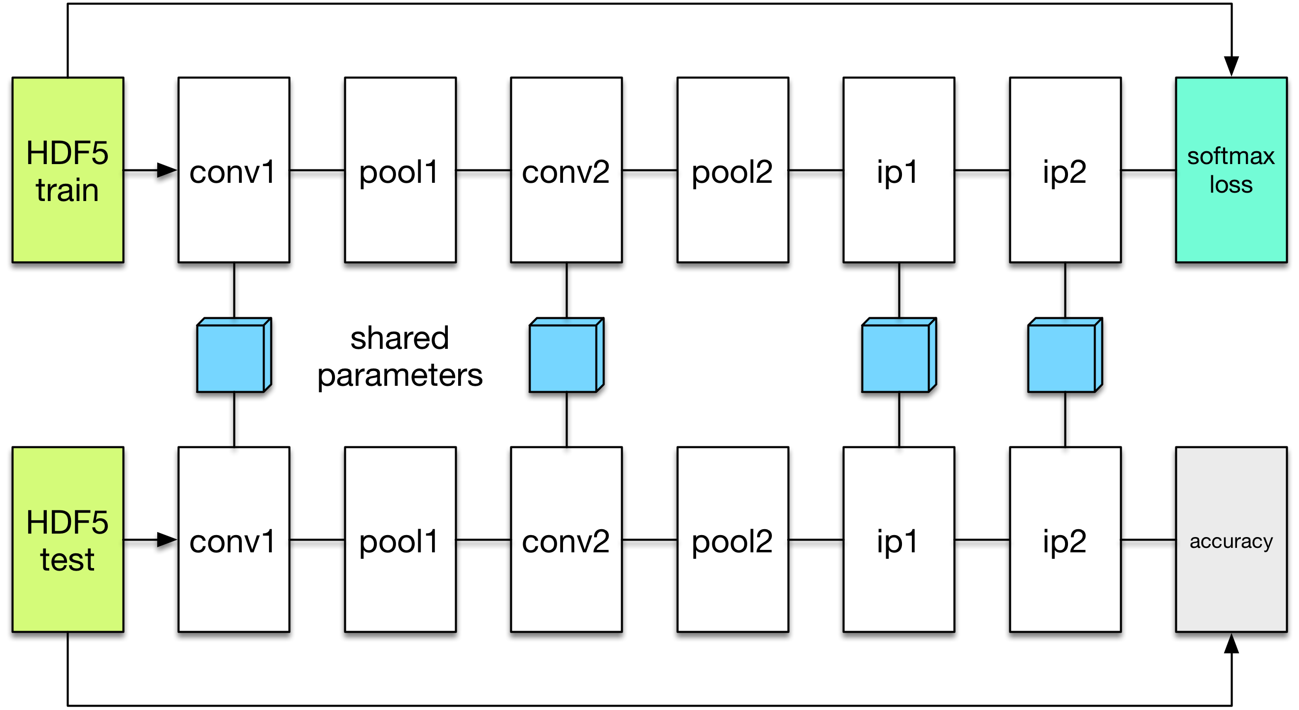
In order to see whether we are really making progress or simply overfitting, we also wish to see the performance on a separate validation set periodically. In this example, we simply use the test dataset as the validation set.
We will define a new network to perform the evaluation. The evaluation network will have exactly the same architecture, except with a different data layer that reads from the validation dataset instead of the training set. We also do not need the softmax loss layer as we will not train the validation network. Instead, we will add an accuracy layer on the top, which will compute the classification accuracy for us.
data_layer_test = HDF5DataLayer(name="test-data", source="data/test.txt", batch_size=100)
acc_layer = AccuracyLayer(name="test-accuracy", bottoms=[:ip2, :label])
test_net = Net("MNIST-test", backend, [data_layer_test, common_layers..., acc_layer])
Note how we re-use the common_layers variable defined a moment ago to reuse
the description of the network architecture. By passing the same layer object
used to define the training net to the constructor of the validation net, Mocha
will be able to automatically setup parameter sharing between the two networks.
The two networks will look like this:
Now we are ready to add another coffee break to report the validation performance:
add_coffee_break(solver, ValidationPerformance(test_net), every_n_iter=1000)
Please note that we use a different batch size (100) in the validation network. During the coffee break, Mocha will run exactly one epoch on the validation net (100 iterations in our case, as we have 10,000 samples in the MNIST test set), and report the average classification accuracy. You do not need to specify the number of iterations here as the HDF5 data layer will report the epoch number as it goes through a full pass of the whole dataset.
Training
Without further ado, we can finally start the training process:
solve(solver, net)

destroy(net)
destroy(test_net)
shutdown(backend)
After training, we will shutdown the system to release all the allocated resources. Now you are ready run the script:
julia mnist.jl
As training proceeds, progress information will be reported. It takes about 10~20 seconds every 100 iterations, i.e. about 7 iterations per second, on my machine, depending on the server load and many other factors.
14-Nov 11:56:13:INFO:root:001700 :: TRAIN obj-val = 0.43609169
14-Nov 11:56:36:INFO:root:001800 :: TRAIN obj-val = 0.21899594
14-Nov 11:56:58:INFO:root:001900 :: TRAIN obj-val = 0.19962406
14-Nov 11:57:21:INFO:root:002000 :: TRAIN obj-val = 0.06982464
14-Nov 11:57:40:INFO:root:
14-Nov 11:57:40:INFO:root:## Performance on Validation Set
14-Nov 11:57:40:INFO:root:---------------------------------------------------------
14-Nov 11:57:40:INFO:root:  Accuracy (avg over 10000) = 96.0500%
14-Nov 11:57:40:INFO:root:---------------------------------------------------------
14-Nov 11:57:40:INFO:root:
14-Nov 11:58:01:INFO:root:002100 :: TRAIN obj-val = 0.18091436
14-Nov 11:58:21:INFO:root:002200 :: TRAIN obj-val = 0.14225903
The training could run faster by enabling the native extension for the CPU backend, or by using the CUDA backend if CUDA compatible GPU devices are available. Please refer to Mocha Backends for how to use different backends.
Just to give you a feeling for the potential speed improvement, this is a sample log from running with the Native Extension enabled CPU backend. It runs at about 20 iterations per second.
14-Nov 12:15:56:INFO:root:001700 :: TRAIN obj-val = 0.82937032
14-Nov 12:16:01:INFO:root:001800 :: TRAIN obj-val = 0.35497263
14-Nov 12:16:06:INFO:root:001900 :: TRAIN obj-val = 0.31351241
14-Nov 12:16:11:INFO:root:002000 :: TRAIN obj-val = 0.10048970
14-Nov 12:16:14:INFO:root:
14-Nov 12:16:14:INFO:root:## Performance on Validation Set
14-Nov 12:16:14:INFO:root:---------------------------------------------------------
14-Nov 12:16:14:INFO:root:  Accuracy (avg over 10000) = 94.5700%
14-Nov 12:16:14:INFO:root:---------------------------------------------------------
14-Nov 12:16:14:INFO:root:
14-Nov 12:16:18:INFO:root:002100 :: TRAIN obj-val = 0.20689486
14-Nov 12:16:23:INFO:root:002200 :: TRAIN obj-val = 0.17757215
The following is a sample log from running with the CUDA backend. It runs at about 300 iterations per second.
14-Nov 12:57:07:INFO:root:001700 :: TRAIN obj-val = 0.33347249
14-Nov 12:57:07:INFO:root:001800 :: TRAIN obj-val = 0.16477060
14-Nov 12:57:07:INFO:root:001900 :: TRAIN obj-val = 0.18155883
14-Nov 12:57:08:INFO:root:002000 :: TRAIN obj-val = 0.06635486
14-Nov 12:57:08:INFO:root:
14-Nov 12:57:08:INFO:root:## Performance on Validation Set
14-Nov 12:57:08:INFO:root:---------------------------------------------------------
14-Nov 12:57:08:INFO:root:  Accuracy (avg over 10000) = 96.2200%
14-Nov 12:57:08:INFO:root:---------------------------------------------------------
14-Nov 12:57:08:INFO:root:
14-Nov 12:57:08:INFO:root:002100 :: TRAIN obj-val = 0.20724633
14-Nov 12:57:08:INFO:root:002200 :: TRAIN obj-val = 0.14952177
Remarks
The accuracy from two different training runs are different due to different random initializations. The objective function values shown here are also slightly different to Caffe’s, as until recently, Mocha counts regularizers in the forward stage and adds them into the objective functions. This behavior is removed in more recent versions of Mocha to avoid unnecessary computations.