Networks

Overview

In deep learning, computations are abstracted into relatively isolated layers. The layers are connected together according to a given architecture that describes a data flow. Starting with the data layer: it takes input from a dataset or user input, do some data pre-processing, and then produce a stream of processed data. The output of the data layer is connected to the input of some computation layer, which again produces a stream of computed output that gets connected to the input of some upper layers. At the top of a network, there is typically a layer that produces the network prediction or compute the loss function value according to provided ground-truth labels.

During training, the same data path, except in the reversed direction, is used to propagate the error back to each layers using chain rules. Via back propagation, each layer could compute the gradients for its own parameters, and update the parameters according to some optimization schemes. Again, the computation is abstracted into layers.

The abstraction and separating layers from architecture are important. The library implementation could focus on each layer type independently, and does not need to worry about how those layers are going to be connected with each other. On the other hand, the network designer could focus on the architecture, and does not need to worry about the internal computations of layers. This enables us to compose layers almost arbitrarily to create very deep / complicated networks. The network could be carrying out highly sophisticated computations when viewed as a whole, yet all the complexities are nicely decomposed into manageable pieces.

Most of the illustrations for (deep) neural networks look like the following image stolen from Wikipedia’s page on Artificial Neural Networks:

When writing Mocha, I found this kind of illustrations a bit confusing, as it does not align well with the abstract concept of layers we just described. In our abstraction, the computation is done within each layers, and the network architecture specifies the data path connections for the layers only. In the figure above, the “Input”, “Hidden”, and “Output” labels are put on the nodes, suggesting the nodes are layers. However, the nodes do not do computation, instead, computations are specified by the arrows connecting those nodes.

On the other hand, I think the following kind of illustration is clearer, for the purpose of abstracting layers and architectures separately:

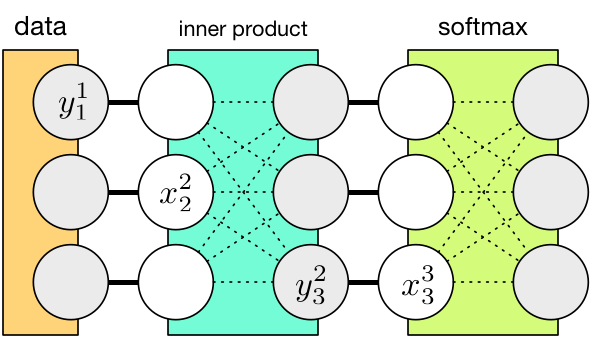
Each layer is now represented as a box that has inputs (denoted by \(x^L\) for the \(L\)-th layer) and outputs (denoted by \(y^L\)). Now the architecture specifies which layer’s outputs connect to which layer’s inputs (the dark lines in the figure). On the other hand, the intra-layer connections, or computations (see dotted line in the figure) should be isolated from the outside world.

Note

Unlike the intra-layer connections, the inter-layer connections are drawn as simple parallel lines, because they are essentially a point-wise copying operation. Because all the computations are abstracted to be inside the layers, there is no real computation in between them. Mathematically, this means \(y^L=x^{L+1}\). In actual implementation, data copying is avoided via data sharing.

Of course, the choice is only a matter of taste, but as we will see, using the latter kind of illustration makes it much easier to understand Mocha’s internal structure and end-user interface.

Network Architecture

Specifying a network architecture in Mocha means defining a set of layers, and connecting them. Taking the figure above for example, we could define a data layer and an inner product layer

data_layer = HDF5DataLayer(name="data", source="data-list.txt", batch_size=64, tops=[:data])
ip_layer   = InnerProductLayer(name="ip", output_dim=500, tops=[:ip], bottoms=[:data])

Note the tops and bottoms properties give names to the output and input of the layer. Since the name for the input of ip_layer matches the name for the output of data_layer, they will be connected as shown in the figure above. The softmax layer could be defined similarly. Mocha will do a topological sort on the collection of layers and automatically figure out the connection defined implicitly by the names of the inputs and outputs of each layer.

Layer Implementation

The layer is completely unaware of what happens in the outside world. Two important procedures need to be defined to implement a layer:

• Feed-forward: given the inputs, compute the outputs. For example, for the inner product layer, it will compute the outputs as \(y_i = \sum_j w_{ij}x_j\).
• Back-propagate: given the errors propagated from upper layers, compute the gradient of the layer parameters, and propagate the error down to lower layers. Note this is described in very vague terms like errors. Given the abstraction we choose here, those vague terms could become very clear.

Specifically, back-propagation is used during network training, when an optimization algorithm want to compute the gradient of each parameter with respect to an objective function. Typically, the objective function is some loss function that penalize incorrect predictions given the ground-truth labels. Let’s call the objective function \(f\).

Now let’s switch to the viewpoint of an inner product layer: it needs to compute the gradients of the weights parameters \(w\) with respect to \(f\). Of course, since we restrict the layer from accessing the outside world, it does not know what \(f\) is. But the gradients could be computed via chain rule

\[\frac{\partial f}{\partial w_{ij}} = {\color{red}{\frac{\partial y_i}{\partial w_{ij}}}}\times {\color{blue}{\frac{\partial f}{\partial y_i}}}\]

The red part could be computed within the layer, and the blue part is the so called “errors propagated from the upper layers”. It comes from the reversed data path as used in the feed-forward pass.

Now our inner product layer is ready to “propagate the errors down to lower layers”, precisely speaking, this means computing

\[\frac{\partial f}{\partial x_i} = \sum_j {\color{red}{\frac{\partial y_j}{\partial x_i}}}\times{\color{blue}{\frac{\partial f}{\partial y_j}}}\]

Again, this is decomposed into a part that could be computed internally and a part that comes from the “top”. Recall we said the \(L\)-th layer’s inputs \(x^L_i\) is equal to the \((L-1)\)-th layer’s outputs \(y^{L-1}_i\). That means what we just computed

\[\frac{\partial f}{\partial x^L_i} = \frac{\partial f}{\partial y^{L-1}_i}\]

is exactly what the lower layer’s “errors propagated from upper layers”. By tracing the whole data path reversely, we now help each layers compute the gradients of their own parameters internally. And this is called back-propagation.